Testing a slime-mould idea against Fisher information
I had a hypothesis. I ran the experiment properly. The hypothesis was wrong, and the way it was wrong turned out to be more interesting than if it had worked.
The problem
Train a neural network on task A, then train it on task B, and it tends to forget A almost entirely. This is called catastrophic forgetting, and it's one of the reasons models are retrained from scratch rather than taught new things incrementally.
One family of fixes works by deciding which weights matter for the old task and gently anchoring those in place while the new task is learned. The whole game is the importance estimate: which weights do you protect?The standard answer is Fisher information (the method called EWC), roughly how sensitive the model's output is to each weight. It works, but it needs an extra gradient computation.
The bet
I wanted to try a different signal, borrowed from biology. Physarum, the slime mould, solves mazes and designs efficient networks with no brain: tubes that carry a lot of flow thicken, tubes that carry little flow wither away. The surviving network isthe solution. The analogue for a neural network: protect the connections that carry the most signal during training. Measure "flow" on the forward pass, no extra gradient needed.
To keep it a fair test I held everything constant except the importance estimate, same model, same anchor penalty, same tasks, and only swapped which signal decides what to protect: naive (no protection), Fisher/EWC, Synaptic Intelligence, and two flow variants. I wrote down my prediction in advance: the flow signal that most resembles the literal slime-mould reading (flow weighted by connection strength) would win.
It worked, on the easy benchmark
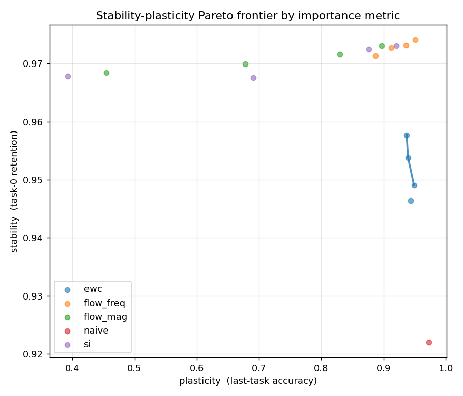
On Permuted MNIST (a deliberately gentle continual-learning benchmark), a flow signal did beat Fisher. But not the one I predicted. The winner was flow-frequency, how often a unit fires, independent of weight strength, while the literal slime-mould version (flow-magnitude) was the worst method of the lot. My pre-registered guess was falsified in the most useful way: the variant that won was the one that couldn't be explained away as just protecting big weights.
| method | stability | plasticity | avg acc |
|---|---|---|---|
| flow-frequency | 0.974 | 0.951 | 0.962 |
| Fisher (EWC) | 0.949 | 0.949 | 0.949 |
| naive | 0.922 | 0.973 | 0.947 |
| flow-magnitude | 0.973 | 0.897 | 0.935 |
Then the hard benchmark broke it
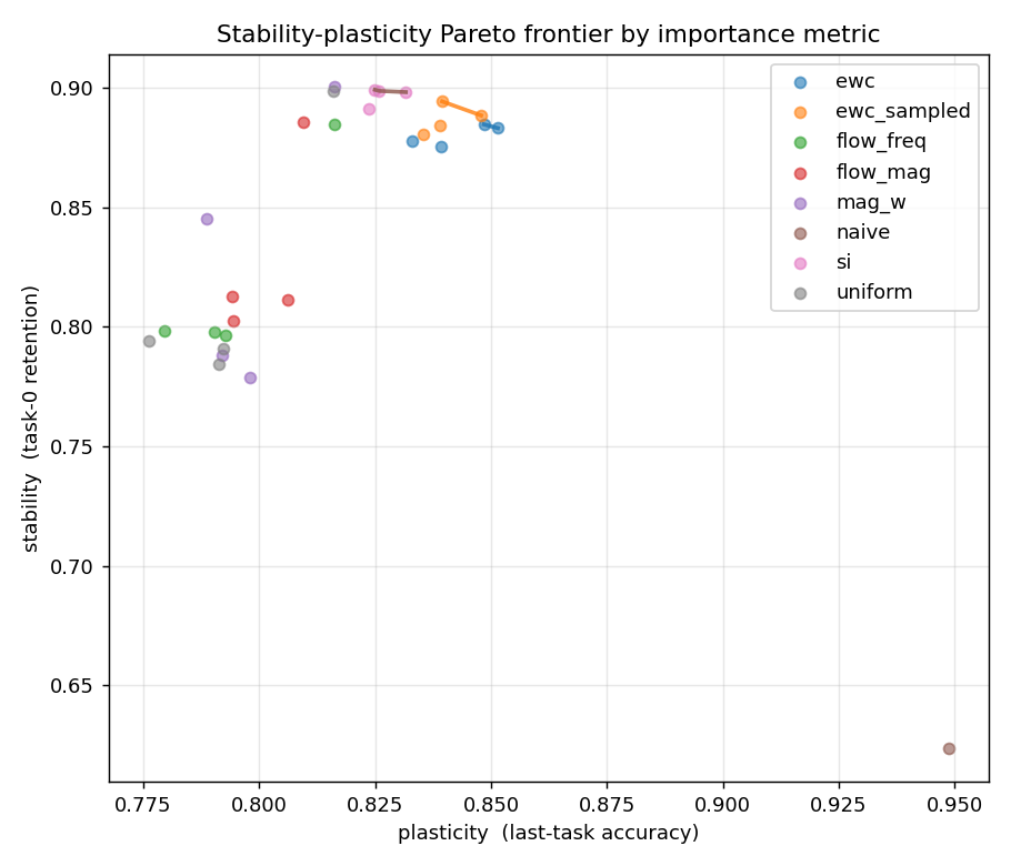
Permuted MNIST is known to be too easy. The real test was Split-CIFAR-10, genuinely different classes per task, a convolutional network. Here the result reversed completely. Flow-frequency dropped to the bottom of the pack: it was statistically indistinguishable from a uniform anchor (protecting everything equally), and it lost to a properly-tuned Fisher in every paired run.
| method | avg acc | |
|---|---|---|
| Fisher (EWC) | 0.822 | wins |
| Synaptic Intelligence | 0.763 | |
| naive | 0.743 | |
| flow-magnitude | 0.736 | |
| flow-frequency | 0.696 | ties "uniform" |
| uniform anchor | 0.695 |
Why, and this is the good part
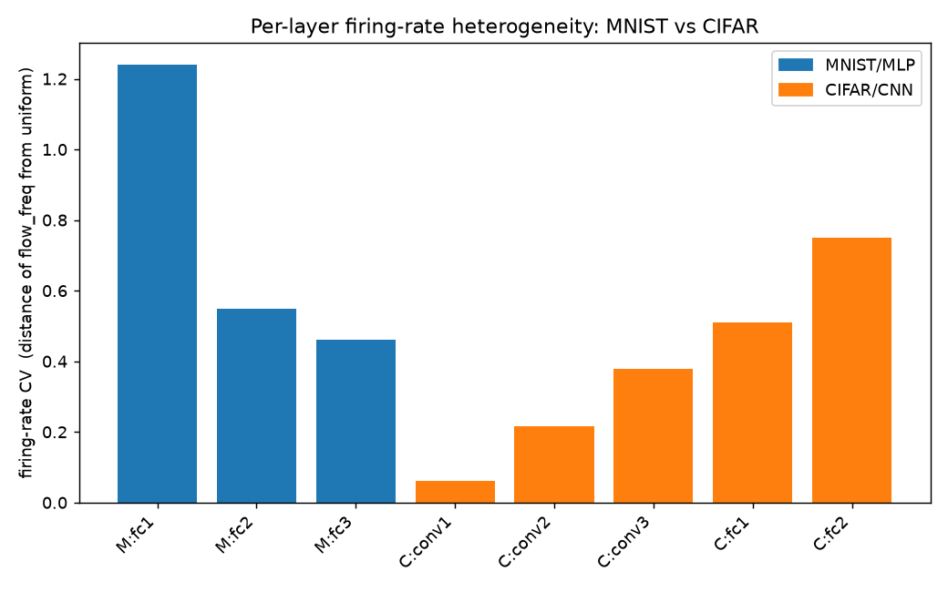
Flow-frequency protects a unit in proportion to how often it fires. That only carries information when firing rates differacross units. MNIST's input pixels are wildly uneven, border pixels almost never fire, central ones often, so the signal is rich. A convolutional network's channels fire much more uniformly, so the same signal flattens into a constant: it becomes the uniform anchor, which is exactly what the CIFAR numbers showed.
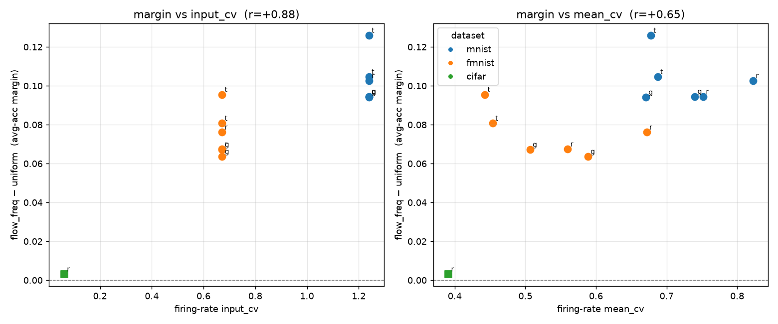
To check this was the actual cause and not a coincidence, I ran a controlled test: take thesameMNIST task and whiten the inputs, which flattens the pixel firing rates without changing the labels. The input heterogeneity collapsed, and on that same task, flow-frequency's edge over Fisher reversed, from +0.02 ahead to −0.21 behind. Homogenise the input and you reproduce the CIFAR failure on MNIST. (The honest caveat: whitening also lowers accuracy across the board, so it's strong corroboration, not an airtight single-variable proof.)
What I take from it
The strong claim, "this biology-inspired signal beats Fisher," is false. The honest, bounded claim that replaced it: forward-pass participation-frequency is a real importance signal, competitive with or better than Fisher when unit firing rates are heterogeneous, and degenerate when they aren't. That's a smaller result than I set out to find, and a more trustworthy one.
I'm writing this up the way it actually went, wrong prediction included, because that's the part most write-ups quietly delete, and it's the part that decides whether you can trust the rest. The same instinct goes into the software I build: pre-register what you expect, test it fairly, and report what happened.
The full write-up (method, all five runs, references) and the code to reproduce every number are on GitHub: reverendish/flow-engram.